
Can Satellites Help Us Understand the Air We Breathe?
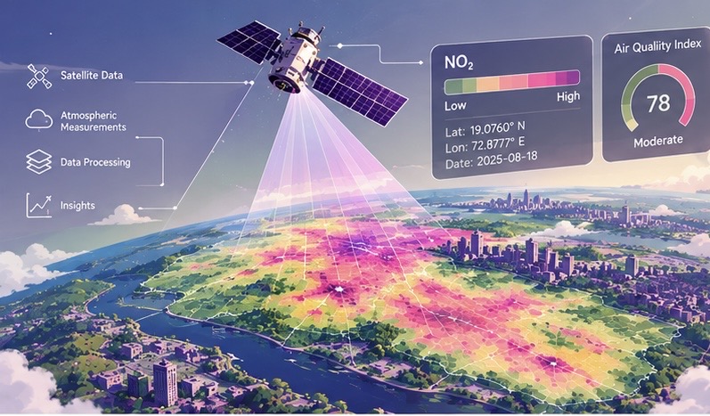
When we think about checking air quality, we usually think of an AQI number on a weather app.
But what if we could examine atmospheric pollution across an entire city from above?
Every day, Earth-observing satellites collect large volumes of information about the atmosphere and surface. Some satellite instruments detect gases and particles by measuring how they absorb, scatter, or emit electromagnetic radiation. These observations can support estimates of pollutant distributions and changes across space and time.
This creates an important question:
Can satellite data help us map and understand air-quality trends in our own cities?
The answer is yes—but satellite observations must be interpreted carefully, and this is where Data Science becomes especially useful.
By combining satellite products with geographic information, ground observations, meteorological data, statistics, and visualization, we can transform millions of measurements into maps and patterns that are easier to analyze.
What Does a Satellite Actually Measure?
Satellites do not simply photograph pollution floating over a city.
Their instruments measure radiance or related properties of sunlight and thermal radiation after it has interacted with the atmosphere and Earth’s surface. Because different gases absorb radiation at characteristic wavelengths, scientists can use these spectral signals in retrieval algorithms to estimate atmospheric composition.
The resulting satellite product may represent different physical quantities depending on the instrument and processing method. For example, it may describe:
- A total or tropospheric atmospheric column amount
- A column-averaged concentration
- An aerosol optical property
- A near-surface estimate derived with additional modeling
- A quality-assurance or uncertainty value
This distinction is essential. A satellite product that reports a pollutant column does not directly measure the concentration at breathing height near the ground. The observation integrates information through part or all of the atmospheric column, whereas a ground monitor samples air at a specific location and elevation, usually near the surface.
Satellite missions can provide information related to pollutants and atmospheric constituents such as:
- Nitrogen dioxide (NO₂)
- Sulfur dioxide (SO₂)
- Carbon monoxide (CO)
- Ozone (O₃)
- Aerosols and particulate pollution
For example, Sentinel-5P is part of the European Union’s Copernicus Earth-observation program. Its TROPOMI instrument measures reflected sunlight in several spectral bands and produces atmospheric composition products at a global scale.
The result is a large geospatial dataset containing estimates of atmospheric properties for specific locations and observation times.
But there is a problem.
A satellite product is not automatically a direct measurement of ground-level air quality.
Its meaning depends on the measured quantity, retrieval method, spatial resolution, vertical sensitivity, atmospheric conditions, and quality controls.
That’s where Data Science enters the picture.
Turning Satellite Measurements Into a Map
Imagine that we want to study air quality in a city.
A satellite dataset might contain thousands of observations covering the city and surrounding areas. Each record can include information such as:
Location → Date and time → Pollutant product → Units → Quality indicators → Other atmospheric variables
Before mapping the data, we need to determine what the pollutant variable represents. For example, a value may be a column density, a column-averaged mixing ratio, an aerosol optical depth, or a modeled surface estimate. These quantities should not be treated as interchangeable.
After selecting appropriate observations and applying quality filters, we can plot the data geographically.
For example:
Lower retrieved values → Intermediate values → Higher retrieved values
Different values can then be represented using different colors or shades on a map.
Suddenly, a table of measurements becomes a visual representation of spatial variation.
We might observe that retrieved pollutant values are higher near certain urban or industrial regions, lower in surrounding areas, or different during particular seasons. However, these patterns describe the satellite product being analyzed; they do not automatically establish the exact pollutant concentration at ground level.
This is one of the most important ideas in Data Science:
Data becomes more useful when we understand both the patterns it shows and the quantity it actually represents.
Why Look at Trends Instead of Just One Day?
A single day’s satellite observation can be informative, but it does not describe the full behavior of a city’s atmosphere.
Suppose a city shows relatively high retrieved NO₂ values on one particular day.
Was that unusual?
Were the observations affected by weather or cloud screening?
Are values normally higher during this season?
Did the long-term pattern change compared with previous years?
To answer questions like these, we need time-series analysis.
We can organize satellite observations by:
- Day
- Week
- Month
- Season
- Year
Then we can calculate averages, compare periods, quantify variability, and visualize changes over time.
For example:
January → February → March → April → May
If the graph shows consistently higher satellite-retrieved values during certain months, that could indicate a seasonal pattern worth investigating. The pattern may reflect changes in emissions, atmospheric transport, sunlight, boundary-layer height, precipitation, or other factors.
Because satellite observations are often affected by cloud cover and retrieval availability, a time series should also report the number of valid observations and, where possible, uncertainty or quality information.
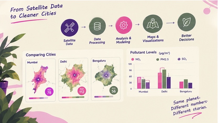
Finding Patterns Across a City
Air pollution is not necessarily distributed evenly across an urban area.
Two neighborhoods within the same city can experience different emissions, atmospheric conditions, and exposure levels.
Areas with heavy traffic, industrial activity, construction, or dense development may show different satellite-retrieved patterns from areas with more vegetation or lower emissions. However, the spatial resolution of a satellite product may be too coarse to distinguish individual streets or neighborhoods, and the observed column may be influenced by pollution transported from outside the city.
With geospatial analysis, we can divide a city into smaller areas and compare them.
For example:
| Area | Average Retrieved NO₂ Product | Possible Context |
| Area A | Higher | Dense traffic |
| Area B | Moderate | Residential |
| Area C | Lower | More open/green space |
| Area D | Higher | Industrial activity |
The values alone do not prove why one area has a higher retrieved product value. They also do not necessarily indicate that people at ground level experienced the same concentration.
However, they can help identify spatial patterns that deserve further investigation.
This distinction is important.
Data can reveal an association, but it does not automatically establish a cause or provide a direct measurement of human exposure.
The Data Science Behind the Map
Creating an air-quality map involves much more than placing satellite pixels on a screen.
A Data Science workflow could look something like this:
Satellite Product → Quality Control → Unit and Variable Interpretation → Spatial Processing → Statistical Analysis → Validation → Visualization → Insights
1. Collect the Data
First, we need satellite observations covering the area and time period we want to study. We should also document the product version, spatial resolution, observation time, units, retrieval method, and relevant quality flags.
2. Clean and Screen the Data
Real-world datasets are rarely perfect.
Some observations may be missing, affected by clouds, influenced by snow or surface reflectance, or flagged as unreliable by the retrieval algorithm. Data cleaning may include removing low-quality pixels, handling missing values, checking units, and recording the number of valid observations used in each summary.
3. Define the Study Area
We can define a geographic boundary around our city and select observations within that region. The choice of boundary matters because urban, suburban, and rural areas may have different emission sources and atmospheric conditions.
4. Interpret and Analyze the Product
Before calculating statistics, we need to identify what the variable measures. We can then calculate statistics such as:
- Mean
- Median
- Minimum
- Maximum
- Standard deviation
- Monthly or seasonal averages
- Observation counts
- Uncertainty or confidence measures, when available
A column measurement, an optical property, and a surface concentration estimate should not be combined without appropriate scientific justification or conversion methods.
5. Compare With Independent Observations
Where possible, satellite products should be compared with ground monitoring stations, meteorological observations, or other independent datasets. This comparison can reveal systematic differences, seasonal biases, and situations in which the satellite product is less representative of surface conditions.
6. Visualize the Results
This is where maps, graphs, and charts become extremely useful.
A map can show the spatial distribution of a satellite-retrieved pollutant product.
A line graph can show how the product changes over time.
A comparison chart can show differences between cities or between satellite and ground observations.
Each visualization should clearly state the variable, units, averaging period, spatial scale, and whether the values represent atmospheric columns or surface concentrations.
Comparing Different Cities
Once the same process is applied to multiple cities, the analysis becomes even more interesting.
Imagine comparing three cities over the same year.
Instead of asking:
“Which city has the highest pollution?”
we can ask more precise questions:
- How do the satellite-retrieved pollutant patterns differ?
- Do the cities experience similar seasonal changes?
- Are spatial hotspots located in similar types of areas?
- How consistent are the trends after accounting for cloud coverage and valid observations?
- Do satellite products and ground monitors show similar temporal behavior?
- Did the retrieved values increase or decrease over time?
This turns a simple dataset into a much larger investigation.
It also demonstrates something important about Data Science:
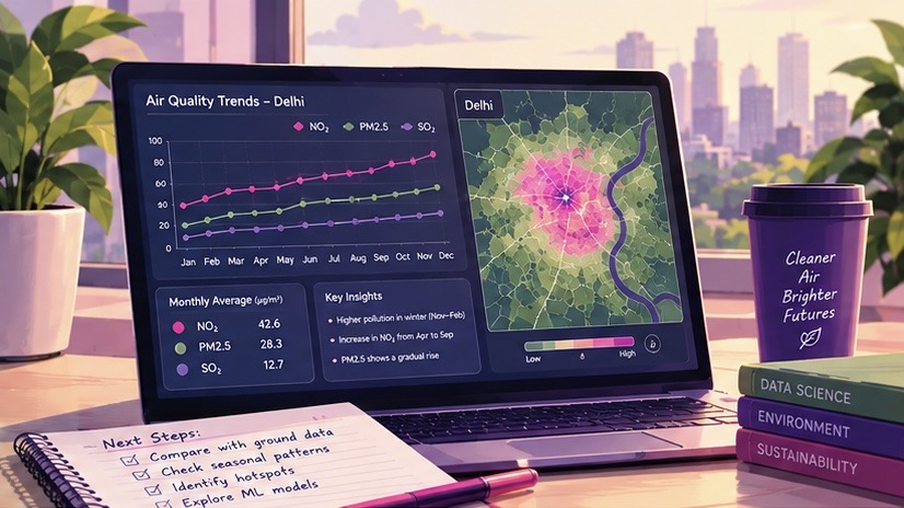
The goal isn’t just to find a number. It’s to understand what the number represents and ask better questions about it.
Satellite Data Has Limitations
Satellites provide broad spatial coverage, but they do not give a complete or direct picture of the air people breathe at every location.
A satellite instrument observes radiation from above and produces a retrieved atmospheric quantity. Depending on the product, that quantity may represent an integrated atmospheric column, a column-averaged value, an aerosol optical property, or a modeled estimate related to near-surface conditions.
A ground monitoring station, by contrast, measures air at a specific site and height near the Earth’s surface. It may measure a surface concentration directly, but only for the location and time represented by the instrument. Therefore, satellite and ground observations are related but not identical measurements.
Differences can arise from:
- Vertical variation in pollutant concentration
- Boundary-layer height and atmospheric mixing
- Clouds and missing observations
- Weather and atmospheric transport
- Surface reflectance and retrieval conditions
- Spatial resolution and representativeness
- Differences in observation time
- Instrument calibration and algorithm assumptions
- Local emissions that are smaller than a satellite pixel
- Differences between column quantities and surface concentrations
For example, a high tropospheric NO₂ column does not necessarily imply the same proportional increase in NO₂ concentration at ground level. The relationship depends on how the pollutant is distributed vertically and on local meteorological conditions.
Because of this, satellite data is often most powerful when combined with other sources.
For example:
Satellite Products + Ground Sensors + Weather Data + Traffic Data + Emissions Information
Together, these datasets can provide a more complete picture of atmospheric composition and surface air quality.
Where Machine Learning Could Come In
Once we have enough historical data, we can go beyond describing satellite-retrieved pollution patterns.
We could explore whether machine-learning models can identify relationships between satellite products, ground-level concentrations, and factors such as:
- Temperature
- Wind speed
- Rainfall
- Boundary-layer height
- Traffic
- Population density
- Industrial activity
- Previous pollution levels
- Cloud and observation conditions
A model could potentially learn relationships between atmospheric columns and surface monitoring data, then estimate near-surface pollution under conditions represented in the training dataset.
However, such estimates depend strongly on the quality and representativeness of the training data. A model trained in one city or season may not perform equally well in another.
Prediction is not the same as certainty.
A machine-learning model gives us an estimate based on patterns in data.
It does not eliminate measurement uncertainty, retrieval uncertainty, sampling gaps, or model bias.
From Maps to Real-World Decisions
Why does all this matter?
Because air-quality data isn’t just about making colorful maps.
Understanding where and when satellite-retrieved pollutant values are higher can help researchers and policymakers investigate important questions.
For example:
- Where should additional monitoring stations be placed?
- Which areas require closer investigation?
- Are satellite and ground observations showing similar changes over time?
- Which seasons show the highest retrieved values or surface concentrations?
- Are environmental policies associated with measurable changes?
- Can satellite products help identify areas that are not adequately represented by existing monitors?
The purpose of Data Science isn’t simply to produce a graph.
It is to interpret measurements carefully and turn multiple data sources into information that can support better decisions.
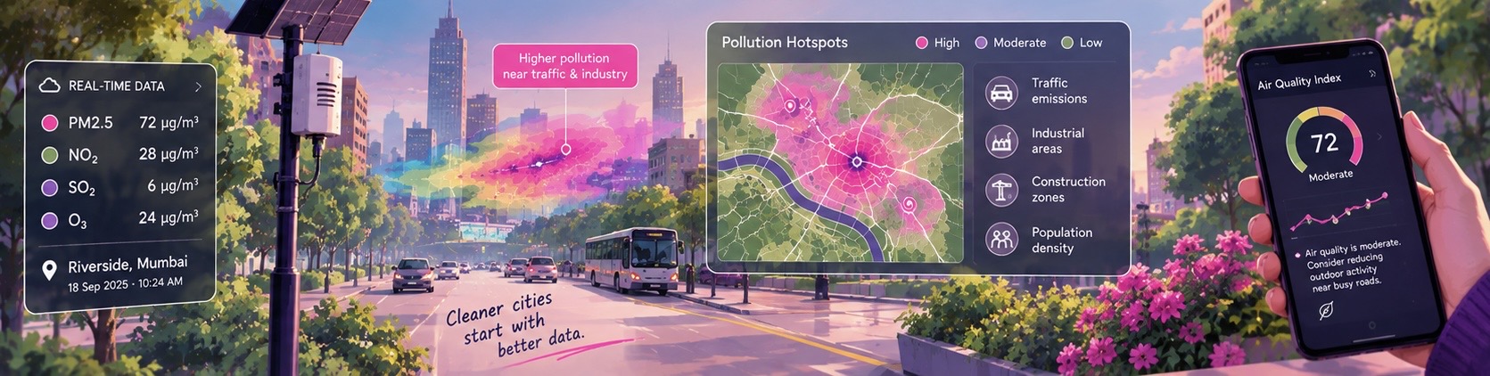
What I Learned From This Idea
What I find most interesting about satellite-based air-quality analysis is how many different areas of Data Science come together in one project.
There is:
Statistics for summarizing measurements and quantifying uncertainty.
Programming for processing large datasets.
Geospatial analysis for understanding location and spatial scale.
Atmospheric science for interpreting columns, surface concentrations, transport, and retrieval conditions.
Data visualization for communicating patterns clearly.
Machine learning for exploring relationships between satellite products and ground observations.
And behind all of this is a real-world problem: the quality of the air we breathe.
This is what makes Data Science interesting to me.
It isn’t only about working with numbers or writing code.
It is about taking a complicated problem, understanding what the measurements represent, combining complementary evidence, and asking whether the data can help us understand the world a little better.
The Bigger Picture
Satellites provide something that traditional measurements alone cannot easily provide: repeated observations of atmospheric patterns across large geographic areas.
But the real power comes from interpreting those observations correctly and combining them with other forms of data.
A satellite observation becomes a scientifically defined product.
A product becomes a quality-controlled dataset.
A dataset becomes a map or time series.
A map reveals a pattern.
A pattern leads to a question.
And that question can lead to further investigation using ground monitors, weather data, emissions information, and atmospheric models.
That is the journey from data to insight.
Air pollution is only one example.
The same approach can be used to study forests, agriculture, water bodies, climate patterns, urban growth, and many other changes happening across our planet.
And perhaps the most exciting part is that these datasets are increasingly accessible—not just to large research organizations, but also to students who want to explore real-world problems through Data Science.
Data is everywhere.
The challenge is learning what it measures, how reliable it is, and how to make sense of it.